Practical 2 : Targeted marketing for predictive analytics
The aim of this practical is to perform a data analysis on the synthetic dataset you generated last week in order to identify a group (or groups) of customers at whom a marketing strategy could be targeted. You will generate summary statistics and data graphics that will characterise what makes your customer groups distinctive from the Leeds population as a whole.
Task 0: Re-visit the datasets
Last week you worked in R and RStudio to create a synthetic population for the c.320,600 households in Leeds using functions contained in the rakeR package. You started with an individual-level survey dataset describing holiday-making behaviours and allocated individuals from this dataset to Output Areas (OAs) in Leeds based on 2011 Census data.
Re-open your .Rproj from last week’s practical. The Environment window in RStudio should list the datasets that you worked upon. Re-familiarise yourslef with these by entering glimpse(<tibble-name>) into the R console.
> glimpse(simulated_oac_age_sex)
Observations: 320,596
Variables: 11
$ person_id            <int> 56, 63, 261, 306, 326, 348, 402, 495, 654, 709, 712, 831,…
$ zone                 <chr> "E00056750", "E00056750", "E00056750", "E00056750", "E000…
$ oac_grp              <fct> 8, 8, 8, 8, 8, 8, 8, 8, 8, 8, 8, 8, 8, 8, 8, 8, 8, 8, 8, …
$ sex                  <fct> m, f, m, m, m, m, m, f, m, m, m, m, m, f, f, f, f, f, m, …
$ age_band             <fct> a65over, a25to34, a25to34, a65over, a50to64, a25to34, a35…
$ number_children      <int> 0, 2, 0, 0, 0, 2, 2, 0, 0, 2, 0, 0, 1, 0, 0, 2, 0, 0, 0, …
$ household_income     <chr> "Not Answered", "26-30K", "26-30K", "Not Answered", "Not …
$ overseas_airport     <chr> "PMI", "FAO", "CUN", "TFS", "PXO", "IBZ", "PMI", "DLM", "…
$ uk_airport           <chr> "MAN", "LBA", "LBA", "MAN", "LBA", "LBA", "MAN", "LBA", "…
$ satisfaction_overall <chr> "poor", "fair", "poor", "excellent", "good", "poor", "poo…
$ age_sex              <fct> m65over, f25to34, m25to34, m65over, m50to64, m25to34, m35…
Create a new RMarkdown file by selecting File > New > New R Markdown..., click OK with the default options, then delete all the placeholder code/text in the new file.
Paste into your RMarkdown file the notes from this document, which contains an outline/skeleton of what you’ll need to complete the practical. Save the file with an appropriate name (practical2).
Task 1: study available variables
This practical session introduces a data analysis to inform a marketing strategyTargeted marketing involves identifying a set of customers that are distinctive in some way and characterising them such that marketing activity could be tailored to them. We are not at all interested in the substantive elements of a marketing strategy in this practical (and module); but rather in the elements of data analysis that could be used to inform and focus strategy development.
. In order to do this, we want to characterise the potential customer population as fully as possible given the data available to us.
Geography is important – where customers of a particular category live and also the types of area in which they live. The simulated dataset allocates individuals to Output Areas (OAs), so we have an indicator of this. These OAs can also be linked to geodemographics.
Demographics clearly play a role – how old and how affluent potential customers are will influence their holiday-making behaviour. In addition to geodemographics, there are known demographic characteristics in the simulated data: sex, age_band, household_income, number_children.
Psychographics is another concept used in targeted marketing, which refers to customer attitudes, aspirations and choices. Psychographics are more difficult to measure because they require some way of ascertaining what people think. In your dataset there are a limited range of these: the destination choice (overseas_airport) suggests something about preference and also how satisfied customers were with their most recent holiday (satisfaction_overall).
Task 1.1: Attach OAC and Airport names
Inspecting the variables in the simulated dataset, you may have noticed that full names are missing for the oac_grp (numeric values rather than supergroup names) and uk_airport and overseas_airport. Lookup tables containing full names are provided as .csv files in the ./data/info directory. We can add these to our simulated dataset, again using dplyr::join.
# Read in lookup tables.
oac_lookup <- read_csv("./data/info/oac_lookup.csv") %>%
  # Cast oac_supergroup as character to join with factor variable in simuldated data.
  mutate(supergroup_code=as.character(supergroup_code))
airport_lookup <- read_csv("./data/info/airport_lookup.csv")

# Join oac names with simulated_oac_age_sex.
# Specify variables on which to join as names not identical.
simulated_oac_age_sex <- simulated_oac_age_sex %>%
  left_join(oac_lookup, by=c("oac_grp"="supergroup_code"))

# Join airport codes names with simulated_oac_age_sex.
# Specify variables on which to join as names not identical.
simulated_oac_age_sex <- simulated_oac_age_sex %>%
  # Do separately for overseas.
  left_join(airport_lookup, by=c("overseas_airport"="airport_code")) %>%
  # Add dest_ prefix so can distinguish destination from origin.
  rename_at(vars(airport_name:airport_country), funs(paste0("dest_",.))) %>%
  # And UK airports.
  left_join(airport_lookup, by=c("uk_airport"="airport_code")) %>%
  # Add orig_ prefix so can distinguish destination from origin.
  rename_at(vars(airport_name:airport_country), funs(paste0("orig_",.)))
Task 1.2: Generate frequency plots
An initial means of exploring how the simulated population distributes on these categorical variables is to plot frequencies across those categories. The code snippet below, also in the .Rmd, displays frequencies of the simulated population amongst each age_band, using ggplot2. {-}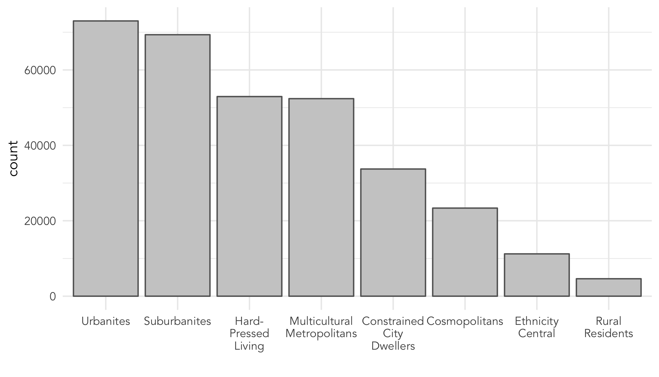
ggplot(data=simulated_oac_age_sex, mapping=aes(x=age_band))+
  geom_bar()
ggplot2 specifications have a consistent form that identifies how data are mapped to visuals:
- Identify dataset :
data= - Specify the mapping :
aes(x=..., y=..., fill=..., ...) - Select a geometry (or marks) layer :
geom_...
Given this, now write ggplot specifications of your own for the other variables in the simulated datasetHint: You will need to change the parameterisation to aes().
.
Task 1.3: Generate frequency plots on variables with many categories
{-}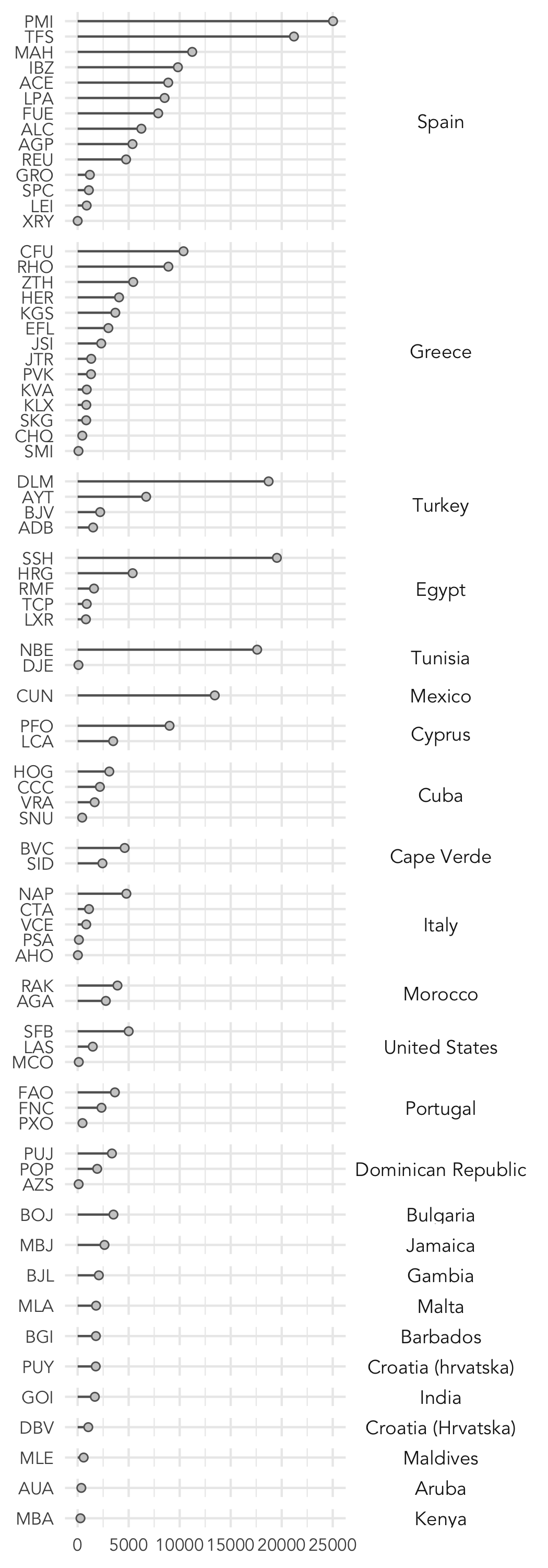
Bar charts are effective at conveying frequencies across categories where the number of levels is reasonably small. You may wish to consider alternatives, such as Cleveland dot plots, for summarising frequencies in data with many levels (destinations in this case).
The code snippet below is a ggplot2 specification for generating a dotplot of frequencies by airport destination. This plot is ordered according to the frequency with which countries are visited, and within countries, the frequency with which airports are visited. In order to effect this ordering, we cast the country variable (dest_airport_country) and airport variable (overseas_airport) as factors and order the factor levels by frequency. There are also some updates to the encodings: since we wish to display frequencies top-to-bottom, airport names (overseas_aiport) are mapped to the y aesthetic (aes()) and frequencies to the x aesthetic, we also use facet() in order to group the plot by destination country.
# Generate tibble of countries ordered by frequency (for ordered factors).
order_country <- simulated_oac_age_sex %>%
  group_by(dest_airport_country) %>%
  summarise(count=n()) %>%
  arrange(-count)

# Cleveland dot plot of destinations, grouped by country.
simulated_oac_age_sex %>%
  # Order dest countries, casting as a factor and ordering levels on frequency.
  mutate(dest_airport_country=factor(dest_airport_country,levels=order_country$dest_airport_country)) %>%
  # Calculate num holidays to each dest airport.
  group_by(overseas_airport) %>%
    summarise(count_airport=n(), dest_airport_country=first(dest_airport_country)) %>%
    # Order by these frequencies.
    arrange(count_airport) %>%
    # Cast as factor and order levels.
    mutate(overseas_airport=factor(overseas_airport,levels=.$overseas_airport)) %>%
  # List airports vertically and frequencies horizontally.
  ggplot(aes(x=count_airport,y=overseas_airport))+
    geom_segment(aes(x=0, y=overseas_airport, xend=count_airport, yend=overseas_airport), colour="#636363")+
    geom_point(colour="#636363", fill="#cccccc", shape=21)+
    # Facet the plot on country to display group freq by destination country.
    facet_grid(dest_airport_country~., scales="free_y", space="free_y")
Task 2: Explore research questions
You now have some knowledge of the data available to you and how the synthetic Leeds population distributes on these key datasets. Next, you should kick-on with your data analysis by identifying research themes and performing exploratory analyses on those themes.
In the example provided here we focus on a single destination, Palma Mallorca (PMI), part of the Balearic Islands, and a destination associated with beach-style holidaysWhen you begin data analysis on your assignment, you should think carefully about the analysis focus. For instance, you may choose to group destinations according to some category – city break, beach holiday, etc. – and characterise the customer populations holidaying to that destination category. You may wish to start with a customer type – for example younger adults without children – and identify destination categories that are accessed by that customer type.
. For a marketing strategy focused on Mallorca, it is clearly useful to profile the known customer population holidaying there (implied by the synthetic population). We will do this in two ways:
- Observing frequencies of known PMI holiday-makers by customer group.
- Comparing these observed frequencies against the frequencies that would be expected given the Leeds holiday-making population as a whole.
Task 2.1: Calculate totals and proportions
You will notice from the Cleveland dotplot that Palma Mallorca is the destination most frequently visited by the synthetic Leeds population. Using some dplyr functions – filter(), summarise() – I calculated a total of 25,030 households holidaying to Palma Mallorca, c.8% of all Leeds households. You may wish to check that a similar figure is recordedDon’t worry if your calculations do not exactly match mine: there is a stochastic element to the procedure we used for running the spatial microsimulation and your synthetic dataset may have been specified with a different set of constraint variables to mine
for your synthetic dataset by writing some code to calculate the total number of households holidaying to Palma Mallorca.
Finding that Palma Mallorca, and destinations in Spain, are those most frequently visited by the synthetic population is fine. Far more interesting and useful is information on the characteristics of the c.8% of households that have visited Palma Mallorca and particularly whether those characteristics are discriminating – e.g. the extent to which they are different from the Leeds population as a whole. The code block below makes use of dplyr functions to calculate:
- The number of Leeds households holidaying to Palma Mallorca by OAC group expressed as a proportion of all holiday-makers to Palma Mallorca
- The number of Leeds households by OAC group expressed as a proportion of all Leeds households
Comparing these numbers allows us to evaluate whether particular OAC groups are over- or under- represented amongst those holidaying to Palma Mallorca.
simulated_oac_age_sex %>%
  # Dummy variable identifying destination to be profiled: PMI.
  mutate(
    # Edit the if_else() to switch focus.
    dest_focus=if_else(overseas_airport=="PMI",1,0),
    total_focus=sum(dest_focus)
  ) %>%
  # Calculate proportions for each OAC group.
  group_by(supergroup_name) %>%
  summarise(
    oac_grp_focus=sum(dest_focus)/first(total_focus),
    oac_grp_control=n()/nrow(.),
    diff_focus_control=oac_grp_focus-oac_grp_control
  )

  # A tibble: 8 x 4
  supergroup_name             oac_grp_focus oac_grp_control diff_focus_control
  <chr>                               <dbl>           <dbl>              <dbl>
1 Constrained City Dwellers          0.157           0.105            0.0513
2 Cosmopolitans                      0.0344          0.0729          -0.0385
3 Ethnicity Central                  0.0127          0.0350          -0.0223
4 Hard-Pressed Living                0.201           0.165            0.0355
5 Multicultural Metropolitans        0.140           0.163           -0.0233
6 Rural Residents                    0.0114          0.0144          -0.00304
7 Suburbanites                       0.216           0.216           -0.000310
8 Urbanites                          0.228           0.228            0.000638
The code above was deliberately written so as to be re-usable. You may wish, for example, to focus on a destination other than Palma Mallorca and profile customers holidaying there. It is possible to do so simply by changing the value with which dest_focus is initialised. For example, if you wanted to focus on Cancun, Mexico (CUN):
simulated_oac_age_sex %>%
  # Dummy variable identifying destination to be profiled: CUN.
  mutate(
    # Edit the if_else() to switch focus.
    dest_focus=if_else(overseas_airport=="CUN",1,0),
    total_focus=sum(dest_focus)
  ) %>%
  ...
  ...
  ...
You may later choose to focus your study on a list of destinations. This can be achieved by generating a vector of destination names and supplying this to dest_focus.
# Create a vector of destination names.
focus <- c("PMI","CFU","DLM")
simulated_oac_age_sex %>%
  # Dummy variable identifying destinations to be profiled: list_focus.
  mutate(
    # Edit the if_else() to switch focus.
    dest_focus=if_else(overseas_airport %in% focus,1,0),
    total_focus=sum(dest_focus)
  ) %>%
  ...
  ...
  ...
Task 2.2: Plot totals and proportions
You will want to profile selected destinations not only on the OAC variables, but by the other demographic and attitudinal variables originally available in the individuals dataset. This could be achieved by re-using the code blocks in the previous section and editing the group_by – e.g. to summarise over the reported satisfaction levels for a given destination group_by(satisfaction_overall).
This would, however, involve much copying-and-pasting of code and here I’ve abstracted the process of calculating proportions grouped on a given variable into my own function. You may have yet to write R functions in LUBS5308, and there are a few syntax things happening here that look odd (!!<parameter-name>)This is to do with the fact that dplyr functions generally use non-standard evaluation, which creates challenges when accessing dplyr programmatically: this post provides an efficient and accessible discussion.
, so do not worry too much about the details here, but a general idea of what the function achieves is useful.
The code snippet below defines the function – on creating this (by running the code), you will notice it listed in the Global Environment window of RStudio:
#' Calculate proportions for a focus and control variable, with user-defined grouping.
#' @param data A df with focus and control variables (focus_var, control_var).
#' @param group_var A string describing the grouping variable passed as a symbol.
#' @return A df of focus and control proportions, with diff values.
calculate_props <-
  function(data, group_var) {
  data %>%
    group_by(!!group_var) %>%
    summarise(
      focus_prop=sum(focus_var)/first(focus_total),
      control_prop=sum(control_var)/first(control_total),
      diff_prop=first(focus_prop)-first(control_prop),
      variable_type=rlang::as_string(group_var)
    ) %>%
    ungroup() %>%
    mutate(variable_name=!!group_var) %>%
    select(-!!group_var)
}
We then create a new dataset that will hold the summary statistics (control and focus proportions) by variable type.
- Create a vector containing the names of grouping variables supplied to
calculate_props(). You can change these variables by editing the fields supplied toselect(). You can also edit the destination(s) to focus on. - Create a new dataset with the control and focus variables (used by
calculate_props()) defined. Note that the control variable is de-facto set to entire population, but you could select a particular subset for comparison here in the same was as the focus variable is defined. - Using a
mapfunction, iterate over each grouping variable name and use this to parameterisecalculate_props().
# Create a vector of the names of grouping variables that will be summarised over.
groups <- names(simulated_oac_age_sex %>%
                  select(supergroup_name, age_band:household_income, satisfaction_overall))
# Identify the destination in focus.
focus <- "PMI"
control <- "ALL"

# calculate_props() requires control and focus variables, not yet contained in
# simulated dataset. Create a new dataset with these added.
temp_simulated_data <- simulated_oac_age_sex %>%
  mutate(
    focus_var=if_else(overseas_airport %in% focus,1,0),
    control_var=1,
    focus_total=sum(focus_var),
    control_total=sum(control_var),
    number_children=as.character(number_children)
 )

# Iterate over each grouping variable, using map_df to bind rows of returned
# data frames.
temp_plot_data <-
 purrr::map_df(groups, ~calculate_props(temp_simulated_data, rlang::sym(.x)))
rm(temp_simulated_data)
Finally plot these data to explore demographic and attitudinal characteristics that are over- or under- represented amongst the destination in focus. I’ve selected Ibiza (IBZ) and the chart does allow us to identify a category of holiday-maker to Ibiza that is discriminating: a bimodal age profile (65+ and 05-49); households with children; Suburbanites OAC groups and not Cosmopolitans.
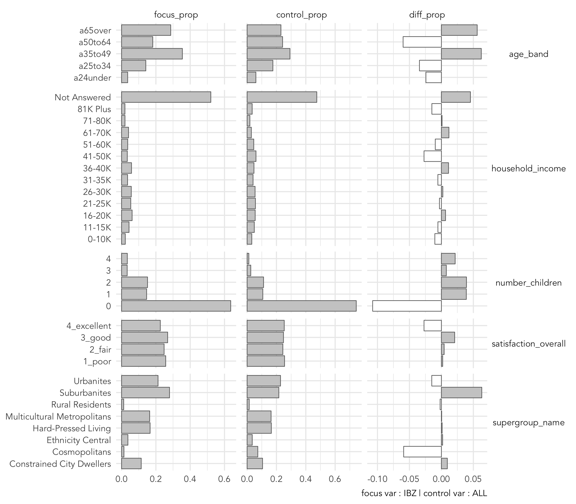
Plot of control and focus proportions
The ggplot2 specification is below, with a little data munging prior to the ggplot2 call:
pivot_longer()thecontrol_prop,focus_prop,diff_dropvariables so that they can be passed tofacet(). These are then identified with thenames_tofield set tostat_type.- In
mutate()caststat_typeas a factor so that the levels can be be ordered in the faceted chart and create a new variablestat_sign, which identifies whetherstat_valueis positive or negative (we do this to differentiate bar colours left and right of the vertical line).
# Define two colours used to colour pos and neg bars differently
fill_colours <- c("#ffffff", "#cccccc")
temp_plot_data %>%
  pivot_longer(names_to="stat_type", values_to="stat_value", -c(variable_type, variable_name)) %>%
  mutate(
    stat_type=factor(stat_type, levels=c("focus_prop","control_prop","diff_prop")),
    stat_sign=stat_value>0
  ) %>%
  filter(!is.na(variable_name)) %>%
  ggplot(aes(x=variable_name, y=stat_value))+
  # stat_sign is a boolean identifying whether stat_value is pos or neg.
  geom_col(aes(fill=stat_sign), colour="#636363", size=0.3)+
  scale_fill_manual(values=fill_colours, guide=FALSE)+
  facet_grid(variable_type~stat_type, scales="free", space="free_y")+
  labs(caption=paste0("focus var : ",focus," | control var : ",control))+
  coord_flip()+
  theme(axis.title=element_blank())
Task 3: Plan your Ass#1 data analysis
This practical provides re-usable code and examples that you could use to perform your Assignment 1 data analysis.
The precise nature and focus of your data analysis is up to you and you should certainly not feel restricted by the techniques made available here. You may wish to explore some machine learning techniques introduced to you as part of your LUBS5308 module: you could for example use decision trees to identify sub-groups of customers associated with a selected destination or set of destinations, CHAID could be a particularly useful technique here; or clustering algorithms to group destination types according to the demographic and attitudinal profile of households holidaying to those locations.
You are not required to use these additional machine learning techniques and only use them if you fully understand them. Your assignment will be marked on the quality and clarity of your data analysis and your ability to make and convey sound analytic thinking.
Some general guidelines for your data analysis:
- Decide on a focus for your study. You may start with a set of destinations and characterise customers and potential customers to those destinations. Or you could start with set(s) of customers and identify candidate destinations for that/those subset(s) (e.g. where do over 65s go on holiday and does this vary by household income?).
- Think carefully how you could aggregate the data: do a range of destinations represent a certain type of holiday?
- Also consider additional variables not discussed in detail during this session. For example, the
satisfaction_overallanduk_airportvariables. Given that this was originally a survey of holiday-makers from Leeds, what might structure in theuk_airportvariable (the airport from which customers leave the country) imply about the behavioural characteristics of a particular sub-group?
End of practical
Well done for completing this week’s practical.
Before you leave the practical make sure you save your work:
- Close your RStudio session by clicking on the red cross in the top left of the window.
- You will be asked to save the changes to the
.Rmdin which you enter code and discussion and a Workspace image with the extension.RData. The.RDatafile stores all data objects (tibbles,ValuesandFunctions) that you have created. Be sure to save both of these.